Part IX: Generative models

Every model in this part answers the same question: given samples \(x^{(1)}, \dots, x^{(N)}\) from a distribution you cannot write down, produce new samples from it. The families differ in how they relate to the density \(p(x)\), and that single choice determines what you can compute, how training behaves, and what a sample costs at inference.

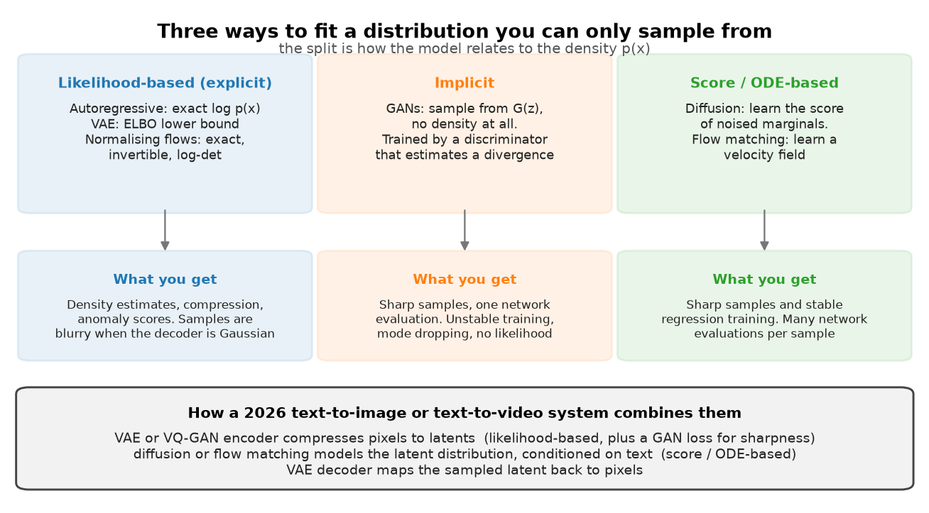
The figure splits the field three ways. Likelihood-based models write down \(p(x)\) or a bound on it, so you get compression, anomaly scores and a loss you can compare across runs. Implicit models define a sampler and nothing else, so you need a second network to say whether the samples look right. Score-based models learn the gradient of the log density of noised versions of the data, which turns generation into a regression problem plus an integrator.

A 2026 image or video system uses all three at once. A VAE or VQ-GAN compresses pixels into a latent grid, trained with a reconstruction loss, a KL or codebook term, and a GAN loss for sharpness. A diffusion or flow-matching Transformer models the latent distribution conditioned on text. The VAE decoder maps the sampled latent back to pixels. Knowing which part of that stack a question is about is half of answering it.

Chapter	The idea you must own	The code you must be able to write
1. Autoencoders and VAEs	The ELBO from two directions, the Gaussian KL in closed form, reparameterisation, posterior collapse as a rate-distortion outcome, VQ-VAE's straight-through estimator.	vae_loss, reparameterize, gaussian_kl_closed_form, VectorQuantizer.
2. GANs	The optimal discriminator \(D^*=p_{data}/(p_{data}+p_g)\), the objective as \(2\,\mathrm{JSD}-\log 4\), why the non-saturating loss exists, what mode collapse looks like.	d_loss_standard, g_loss_non_saturating, gradient_penalty, one alternating training step.
3. Diffusion	\(q(x_t\mid x_0)\) in closed form, the ELBO collapsing to \(\lVert \varepsilon - \varepsilon_\theta \rVert^2\), the posterior mean, DDIM, v-prediction, classifier-free guidance, latent diffusion.	q_sample, ddpm_loss, posterior_mean_variance, sample_ancestral, sample_ddim, predict_eps_cfg.
4. Flow matching	Conditional flow matching and why regressing the conditional velocity has the same gradient as the marginal one, rectified flow, the link to diffusion.	linear_path, cfm_loss, sample_euler.

Prerequisites

• Probability for change of variables, Gaussian algebra and conditioning. Chapter 1 uses the Gaussian KL, chapter 3 uses the product of two Gaussians.
• Information theory for KL divergence, Jensen's inequality and the rate-distortion framing that explains posterior collapse.
• Backpropagation for the straight-through estimator and for why a sampling step blocks gradients until you reparameterise it.
• Attention mathematics for the cross-attention conditioning in latent diffusion and for DiT.
• CLIP and contrastive learning for the text encoder that conditions every text-to-image model here.
• Evaluation for FID, Inception Score and their failure modes, which chapter 2 uses and chapter 3 relies on.

If you have one day

1. Chapter 1, sections 2 and 3 (both ELBO derivations, the Gaussian KL, reparameterisation, the VQ straight-through trick), 2 hours. Retype vae_loss and VectorQuantizer.forward.
2. Chapter 3, sections 2 and 3 up to ancestral sampling, 3 hours. This is the highest-yield block in the part. Retype q_sample, ddpm_loss, posterior_mean_variance, sample_ancestral.
3. Chapter 3, sections on DDIM, v-prediction and classifier-free guidance, 1.5 hours. Derive the CFG formula on paper.
4. Chapter 4, sections 1 to 3, 1.5 hours. Retype cfm_loss and sample_euler.
5. Chapter 2, sections 2 and 4 (optimal discriminator, JSD, failure modes), 1 hour. Read only.

Chapter 2 is last on purpose. GANs are asked about as literacy and as the adversarial loss inside a VQ-GAN tokeniser, not as something you are likely to train in 2026.

Where this part is used later

• Part X: denoising and masking as pretext tasks are the same corruption idea that chapter 1 introduces and chapter 3 industrialises.
• Part XI, world models: driving world models are conditional video diffusion models.
• Part XIII, evaluation: FID, CLIP score and human preference evaluation for generative systems.
• Part XIV, inference systems: a 30-step sampler is 30 forward passes, which changes every serving decision.

Code map

All Part IX code lives in src/mlbook/generative/ and is tested by tests/test_generative_*.py (python -m pytest tests/test_generative_* -q):

Module	Contents
toy_data.py	2-D mixtures and two-moons samplers shared by every chapter, plus a manifold-distance metric
autoencoder.py	MLP autoencoder, Gaussian and masking corruptions, the denoising objective
vae.py	VAE, reparameterize, closed-form and Monte-Carlo Gaussian KL, vae_loss with the decoder scale
vqvae.py	VectorQuantizer with straight-through gradients, commitment loss, codebook perplexity
gan.py	generator, discriminator, standard/non-saturating/Wasserstein losses, gradient penalty, spectral norm by power iteration
ddpm.py	schedules (linear, cosine, zero terminal SNR), q_sample, parameterisation conversions, posterior, EpsMLP, ancestral and DDIM samplers, CFG
flow_matching.py	VelocityMLP, linear and Gaussian probability paths, cfm_loss, Euler and midpoint samplers, exact and Hutchinson divergence

What interviewers actually ask

Four questions cover most of this part.

1. Derive the ELBO and explain each term. Then: what is the reparameterisation trick for, and what breaks without it.
2. Write the DDPM training loop on a whiteboard. Then: why does the simplified loss drop the weighting from the ELBO, and what does that weighting do.
3. Explain classifier-free guidance, including the formula, and what happens as the scale grows.
4. Your text-to-image service costs too much per image. List the levers. (Fewer steps via DDIM or a distilled model, a smaller latent grid, batching, caching the text encoder, a lower guidance scale so you can drop the unconditional pass.)